Stochastic Optimization

Introduction

Calibration of measurement instruments such as sensor systems and sensor networks is the process of relating sensor readings to desired units. If mobile references are available, measured values can be synchronized between devices during encounters. This was one of the ideas of Calibree, which interpreted calibration as a filtering problem, estimating the deviation between calibrated and uncalibrated devices in a stochastic way. Calibration is, however, also a supervised learning problem. From this perspective, the field of gradient-based optimization opens up. As a consequence, modern approaches for online learning that are more flexible can be applied. The following post looks at the theoretical aspects and motivates stochastic online calibration.

Linear Models

Once a data set $\mathbf{X} = [\mathbf{x}_1, …, \mathbf{x}_p] = [x_1, …, x_n]^T \in \mathbb{R}^{n\times p}$ in $n$ samples and $p$ independent variables (or features) $X_i \in \mathcal{X}$, $i\in{1, …, p}$ is collected (with $n > p$), the influence of the independent variables on the dependent variables $Y_k \in \mathcal{Y}$, $k\in{1, …, q}$ can be evaluated. In this notation, $\mathbf{X}$ contains a column with 1’s for the intercept. The aim is to find a function $f$ that maps from $\mathcal{X}$ to $\mathcal{Y}$, i.e., $f: \mathcal{X}\to\mathcal{Y}$. This is a supervised learning problem because the output is known. If the output is also continuous ($Y \in \mathbb{R}$), this particular type of task is called regression. For instance, calibrating a low-cost sensor system is a typical regression problem.

Let the vector $\mathbf{y} = [y_1, …, y_n]^T \in \mathbb{R}^{n}$ be the noisy realization of $Y$ generated by the model $\mathbf{y} = \phi(\mathbf{X}w) + \boldsymbol\epsilon$ with $\epsilon_i \sim \mathcal{N}(0, \sigma^2)$ for $i \in {1, …, n}$, $w \in\mathbb{R}^{p}$ the model parameters, and $\phi(\cdot)$ an activation function. For the identity activation function $\phi(z) = z$, the model becomes $\mathbf{y} = \mathbf{X}w+\boldsymbol\epsilon$. As there are some degrees of freedom, the solution to this system of equations, $\hat{w}$, is obtained by minimizing the sum of squared differences between the the predicted (i.e., model output) and the observed values in Eq. \ref{mse}.

\begin{equation} \label{mse} \hat{w} = \arg \min_{w} \underbrace{(\mathbf{y}-\mathbf{X}w)^T(\mathbf{y}-\mathbf{X}w)}_{\mathcal{L}(w)} \end{equation}

The loss function $\mathcal{L}$ can be motivated from an algebraic perspective by seeking a suitable basis in $\mathcal{X}$ for the expression of vector $\mathbf{y}$ (projection onto $\mathcal{X}$), but it also arises when minimizing the negative logarithmic likelihood of the observed data. The framework is known as linear regression because it is linear with respect to the model parameters (but not the linear activation function or variables). The closed-form solution is obtained by differentiating with respect to $w$ and setting the derivative to zero; it is given by Eq. \ref{lin_reg_sol}.

\begin{equation} \label{lin_reg_sol} \hat{w} = (\mathbf{X}^T\mathbf{X})^{-1}\mathbf{X}^T\mathbf{y} \end{equation}

Gradient-Based Optimization

Solving the system in this manner is not always possible because an analytical solution does not exist in every case. Fortunately, the problem is also solvable in an iterative manner by means of gradient descent (Fig. 1). The main idea is to move along the loss landscape towards the steepest direction (i.e., the gradient) in small steps $t$ until reaching an optimum (Eq. \ref{sgd1}).

\begin{equation} \label{sgd1} w_{(t+1)} \gets w_{(t)} - \gamma\left.\frac{\partial \mathcal{L}}{\partial w}\right\vert_{w=w_{(t)}} \end{equation}

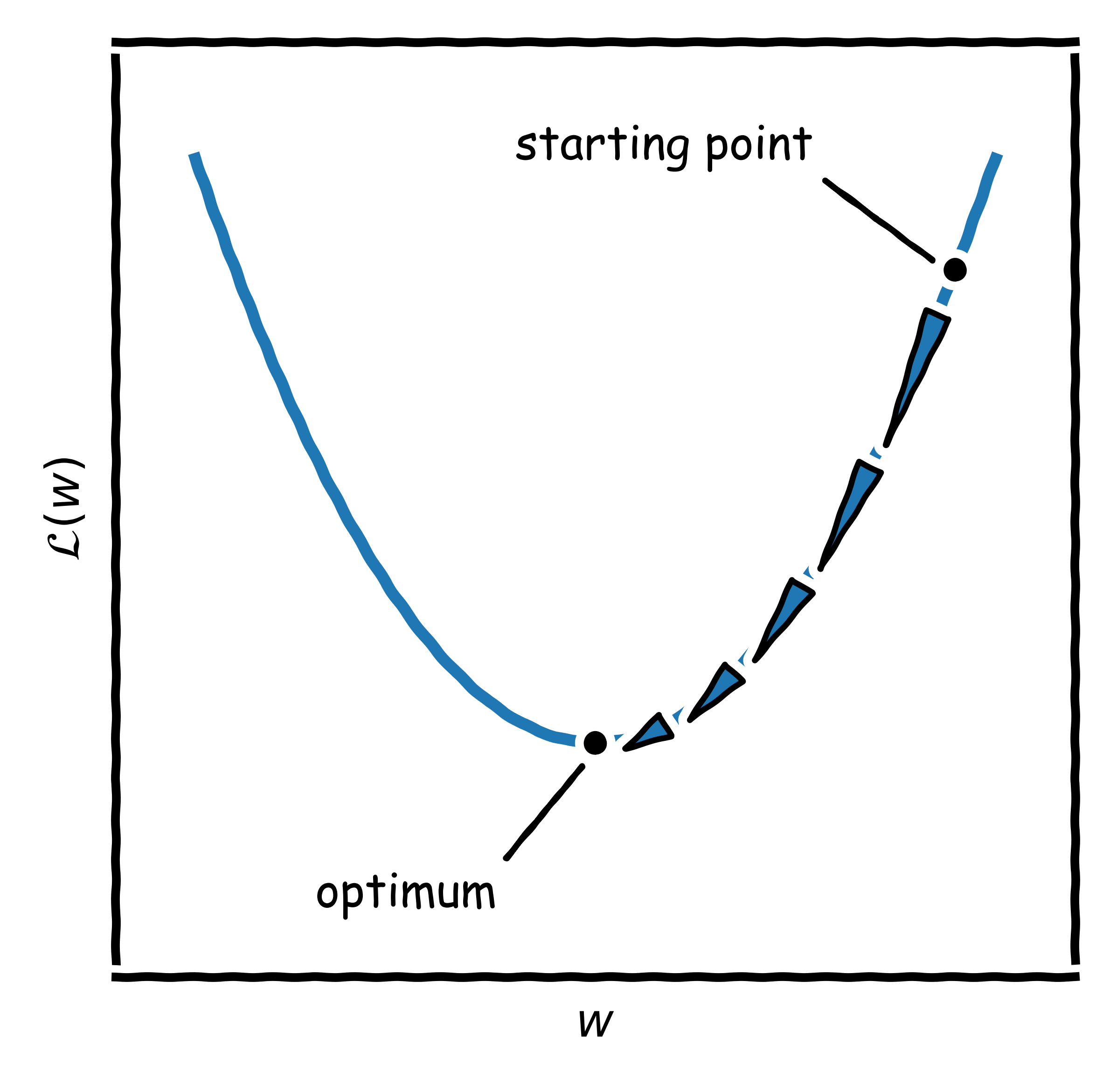
To do so, the objective function must be differentiable; also, a starting point $w_{(0)}$ and a learning rate $\gamma$ are required. For a linear model, the update rule in Eq. \ref{sgd2} is then applied until convergence.

\begin{equation} \label{sgd2} w_{(t+1)} \gets w_{(t)} - \gamma\mathbf{X}^T(\mathbf{y}-\mathbf{X}w_{(t)}) \end{equation}

Instead of using the complete data set of $n$ samples, a mini-batch or only the $k$-th random sample $x_{k}^T$ can be picked and the update is performed only with instance. This is known as stochastic gradient descent. Updating parameters with single observations is reasonable in situations in which new data are becoming available, i.e., in online learning, and when models need to be updated due to changes in the underlying probability distributions.

Neural Networks

If the underlying relationships are non-linear, it is beneficial to add additional variables to $\mathbf{X}$ via basis expansion (i.e., $X_i^2$, $X_iX_j$, and so on). If interpretability is not crucial, one can apply a cascade of $L-1$ non-linear transformations instead, e.g., the sigmoid $\phi(z) = \frac{1}{1+e^{-z}} = \sigma(z)$, and a last affine (“linear”) transformation, each parameterized by a set of parameters $\mathbf{W}^{[l]} \in \mathbb{R}^{n_{l}\times n_{l-1}}$ for transformation $l$ (Eq. \ref{nn}).

\begin{align} \mathbf{y}^T = \phi_{\mathbf{W}^{[L]}} \circ \phi_{\mathbf{W}^{[L-1]}} \circ … \circ \phi_{\mathbf{W}^{[1]}}(\mathbf{X}^T) +\boldsymbol\epsilon^T \label{nn} \end{align}

The approach is supported by an universal approximation theorem and the resulting model is known as multilayer perceptron or feedforward artificial neural network (Fig. 2).

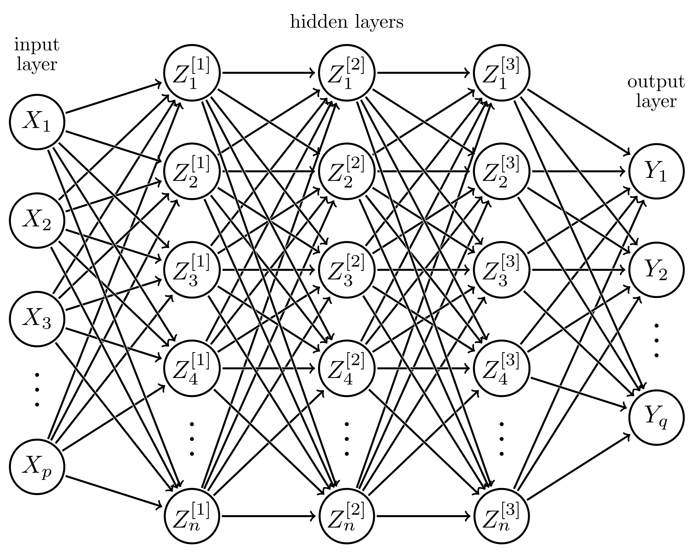
The variables $L$ and $n_l$ for $l\in{1, … , L-1}$ are design parameters. Decomposing the expression from above, with $\mathbf{Z}^{[0]} = \mathbf{X}^T$ and $\mathbf{Z}^{[L]} = \mathbf{y}^T$, results in the intermediate values $\mathbf{Z}^{[l]}$ of the hidden nodes in layers $l\in {1, …, L}$. Eqs. \ref{nn1} & \ref{nn2} are the so-called forward pass.

\begin{align} \label{nn1} \mathbf{A}^{[l]} = \mathbf{W}^{[l]}\mathbf{Z}^{[l-1]} \end{align}

\begin{align} \label{nn2} \mathbf{Z}^{[l]} = \sigma(\mathbf{A}^{[l]}) \end{align}

The loss (Eq. \ref{mse}) remains but an analytical solution does not exist. The algorithm to optimize the model parameters is a variant of gradient descent (with an excessive use of the chain rule) known as backpropagation. Eqs. \ref{backprop1} & \ref{backprop2} describe the backward pass.

\begin{align} \label{backprop1} \frac{\partial \mathcal{L}}{\partial \mathbf{W}^{[l]}} = \frac{\partial \mathcal{L}}{\partial \mathbf{Z}^{[L]}} \frac{\partial \mathbf{Z}^{[L]}}{\partial \mathbf{A}^{[L]}} \frac{\partial \mathbf{A}^{[L]}}{\partial \mathbf{Z}^{[L-1]}}… \frac{\partial \mathbf{A}^{[l]}}{\partial \mathbf{W}^{[l]}} \end{align}

\begin{align} \label{backprop2} \mathbf{W}^{[l]} \gets \mathbf{W}^{[l]} - \gamma \frac{\partial \mathcal{L}}{\partial \mathbf{W}^{[l]}} \end{align}

Bias-Variance Trade-Off and Regularization

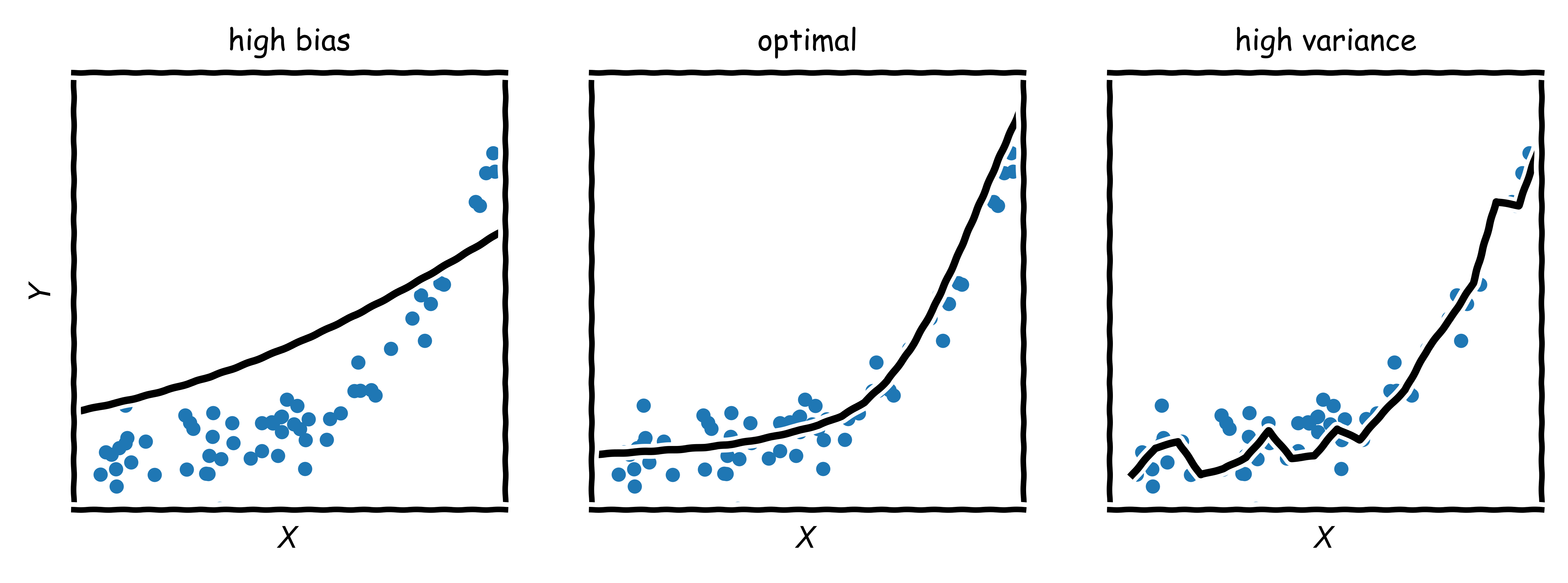
The central problem in frequentist statistics is that the collected data are random and all deduced quantities, such as the estimated function $\hat{f}(x)$, are thus random as well. Very deep or wide neural networks, for instance, can have large model capacity and are able to express quite complex relationships between inputs and output; on one side, however, the estimated function might vary significantly around its expected value $\text{E}[\hat{f}(x)]$ upon exchange of data followed by re-estimation (e.g., because it fits the noise). On the other side, the model capacity might also be insufficient (e.g., because not all variables that would be theoretically necessary for a good fit are part of the model); as a consequence, the outputs of $\hat{f}(x)$ could be far away from the observed values $y=f(x)+\epsilon$ (with $\text{E}[\epsilon] = 0$) generated by the true model $f(x)$. In summary, the estimated function $\hat{f}(x)$ could be too simplistic, too complex, or optimal (Fig. 3).

More formally, the expected squared difference (mean squared error) $\Delta^2$ between observed $y=f(x)+\epsilon$ and predicted $\hat{f}(x)$ is given by Eq. \ref{biasvariancetradeoff}.¹

\begin{equation} \Delta^2 = \sigma^2_{\epsilon} + \text{E}[f-\hat{f}]^2 + \text{E}[(\hat{f}-\text{E}[\hat{f}])^2] \label{biasvariancetradeoff} \end{equation}

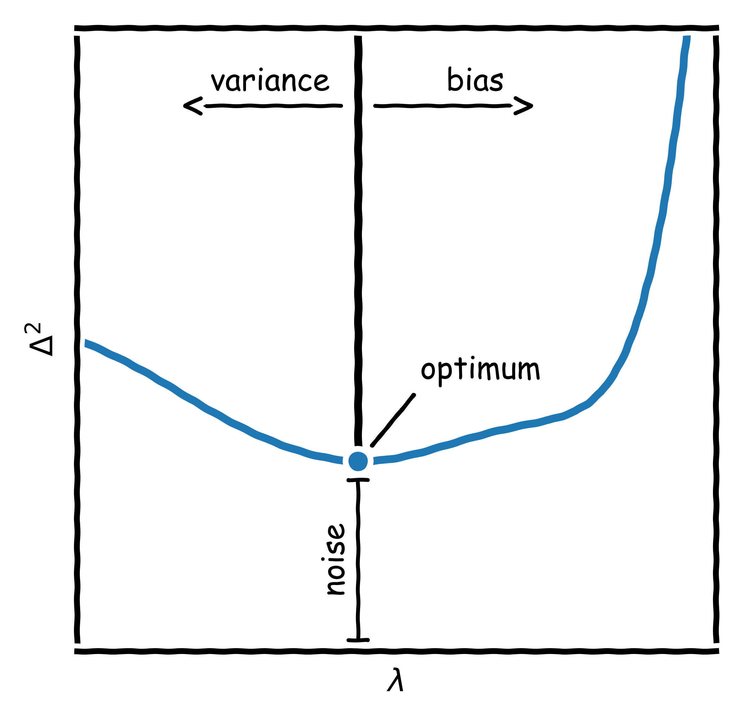
This derivation shows that there are three components to $\Delta^2$: the irreducible noise, the squared bias (deviation from the true value), and the variance (variability around the expected value). If there is a large contribution from the bias, the model is too simplistic and is “underfitting”; if the contribution stems mainly from the variance, the model is too complex and is “overfitting”. The lowest possible error is the inherent noise in the data. Intuitively, it seems that the middle subplot depicts the correct model, and the question arises how to get to it. The solution is called regularization and the idea is to penalize the magnitude of the parameter vector $w$ in the loss from Eq. \ref{mse}, controlled by a hyperparameter $\lambda$ (Eq. \ref{regularization}).

\begin{equation} \label{regularization} \hat{w} = \arg \min_{w} \mathcal{L}(w) + \lambda w^Tw \end{equation}

This regulates the complexity as the magnitude of $w$ contributes to the loss so that explaining observations has a cost. For large values of $\lambda$, solutions with low values of $w$ will be preferred (and vice versa). The next question that arises is how to choose the value of $\lambda$ (as directly optimizing for it results in $\lambda = 0$). For this purpose, cross-validation has been developed. It requires splitting the observations into $B$ equally sized sets; training the model with $B-1$ sets; and calculating $\Delta^2$ for the remaining set; this is done for all $B$ sets and different values of $\lambda$. The value of $\lambda$ associated with the lowest $\Delta^2$ leads to the optimal model complexity (Fig. 4).