Robust Covariance

Introduction

Connectivity (i.e., the internet of things) combined with machine learning are enablers of interesting applications such as predictive maintenance, i.e., autonomously assessing the condition of equipment in order to estimate when maintenance should be performed. For this purpose, it is important to have mathematical models that can distinguish between “normal” and “non-normal” behavior of the equipment, a task called anomaly detection. Equipped with all kinds of sensors, a machine or device can use this collection of sensor data (e.g., temperature, fan speed, pressure, flow rate, etc.) to assess its state and call for service if necessary; the more its behavior deviates from its reference state just after fabrication, the more it will need maintenance.

Mahalanobis Distance

In statistics, deviation can be assessed by the $Z$-score. The generalization of the $Z$-score for a point $x$ in the case of a $p$-dimensional multi-variate probability distribution with some mean $\mu$ and covariance matrix $\Sigma$ is known as Mahalanobis distance $d$, which is given by Eq. \ref{Mahalanobis}.

\begin{equation} d = \sqrt{(x - \mu)^T \Sigma^{-1} (x - \mu)} \label{Mahalanobis} \end{equation}

This metric assesses how many standard deviations $\sigma$ away point $x$ is from $\mu$, thereby being dimensionless. An extreme observation has a large distance from the center of a distribution. It is useful in predictive maintenance as it enables finding unusual behavior of a system; upcoming down-times and malfunction can be targeted and identified, which is particularly important since finding faults in equipment, machines, and devices early can reduce the extent of the damage.

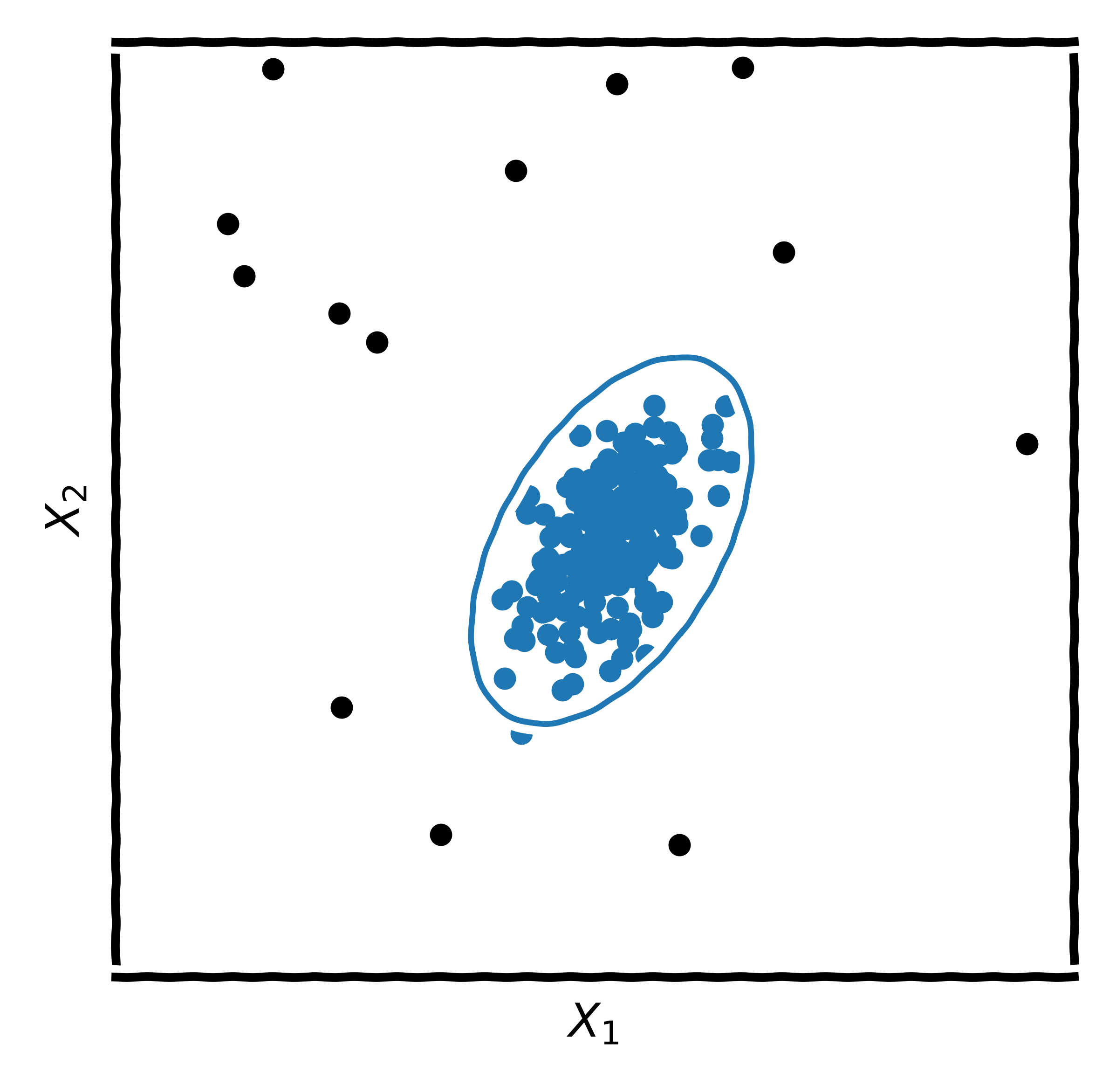
Given a data set $\mathbf{X}$ with $n$ samples in $p$ variables (i.e, data from $p$ sensors), mean and covariance matrix are easily computed. However, in the presence of outliers, both are distorted and the Mahalanobis distance is rendered useless, hence a robust method, i.e., a method that is little affected by outliers, would be desired. In Fig. 1, the support of a Gaussian distribution for some two-dimensional sensor data set $\mathbf{X}$ is plotted; just like with the $Z$-score (e.g., $\pm 1.96\sigma$), an envelope around the data set can be constructed by choosing a critical value of the Mahalanobis distance. Points outside this envelope are considered anomalies/outliers.

Robust Covariance

Robust covariance methods are based on the fact that outliers lead to an increase of the values (entries) in $\Sigma$, making the spread of the data apparently larger. Consequently, the determinant $|\Sigma |$ will also be larger, which would theoretically decrease by removing extreme events. Rousseeuw and Van Driessen developed a computationally efficient algorithm that can yield robust covariance estimates. Their method is based on the assumption that at least $h$ out of the $n$ samples are “normal” ($h$ is a hyperparameter). The algorithm starts with $k$ random samples with $p+1$ points. For each of the $k$ samples, $\mu$, $\Sigma$, and $|\Sigma |$ are estimated, the distances are calculated and sorted in increasing order, and the $h$ smallest distances are used to update the estimates. In their original publication, the subroutine of computing distances and updating the estimates of $\mu$, $\Sigma$, and $|\Sigma |$ is called a “C-step”. They figured out that two such steps are sufficient to find good candidates (for $\mu$ and $\Sigma$) among the $k$ random samples. In a next step, a subset of size $m$ with the lowest $|\Sigma |$ (the best candidates) is considered for computation until convergence, and the one estimate whose $|\Sigma |$ is minimal is returned as output.

Note that the squared distance $d^2$ follows a $\chi^2$-distribution with $p$ degrees of freedom. To compute a critical distance (threshold) for the envelope, a quantile, i.e., the probability of observing a squared distance as extreme as the threshold — also known as p-value — is chosen, and the critical distance is then computed from the inverse cumulative distribution. (For one variable and a probability threshold/p-value of $0.05$, the critical $\chi^2$ value is $3.84$, which corresponds to the squared distance; the square root of that is $1.96$, which is consistent with the intuition for one dimension, e.g., from statistical tests.)

This algorithm is implemented in the elliptic envelope class of scikit-learn. Its most important hyperparameter is the amount of contamination $\nu$, which is related to the parameter $h$ in the original algorithm, since $\nu = 1-\frac{h}{n}$. This hyperparameter has to be tuned to obtain the desired performance.

Non-Parametric Methods

The Mahalanobis distance is a simple and intuitive method that can perform well when the data is close to normally distributed. In other cases, the envelope might be not fit perfectly around the data, which is why non-parametric methods such as one-class support vector machine or isolation forest have been developed. In practice, different algorithms have to be evaluated — including hyperparameter optimization. Embedding these models in machines and devices can bring a lot of added-value and lead to competitive advantage, now it is up to research and development engineers/managers to spot such opportunities.