Design of Experiments
16 August 2022

Introduction
Experiments are essential when exploring systems.1 They generate data that can be used to evaluate relationships between variables. However, care is needed in the design, as undesirable correlations (i.e., non-orthogonality) between variables can lead to false conclusions. In addition, the workload explodes with too many variables. This article explains how to get rid of such problems.
Full Factorial Design
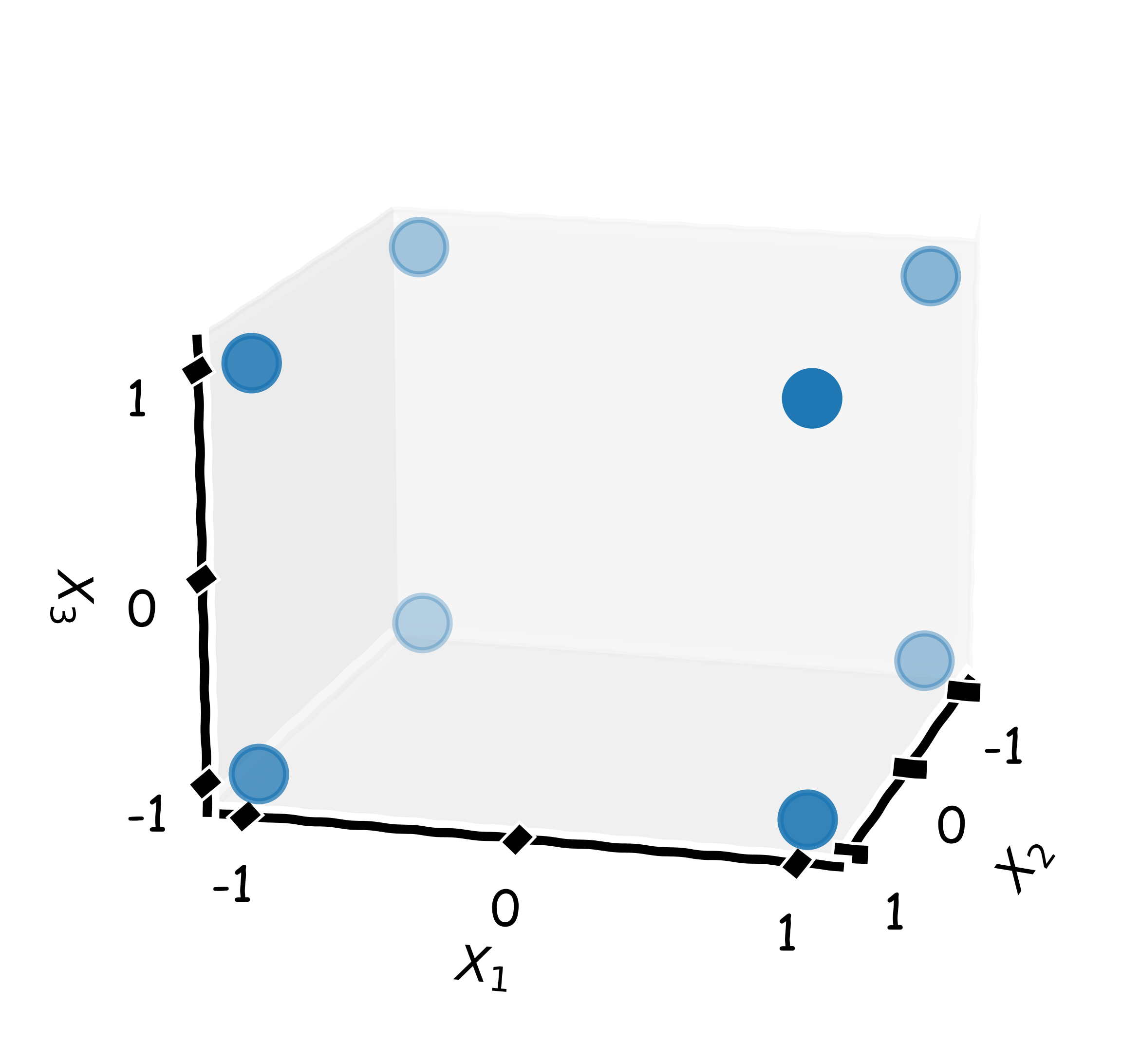
The most basic experimental design, the “full factorial”, includes samples of $k$ variables at $n$ levels, resulting in $n^k$ data points, which is only feasible for few variables and levels as otherwise the number of experiments becomes too large. Furthermore, due to this poor scaling of the workload, the number of levels is limited to two (or three) in most applications, usually coded as $-1$ and $+1$, corresponding to an interval from low to high “expression”.
Thus, it is also known as $2^k$ full factorial design (Fig. 1a). With only two levels per variable, it is not possible to include power terms in a model. In some situations, e.g., if the noise is high, it might be reasonable to replicate all runs. A design is stored as matrix $\mathbf{X}$ in which each row $x^T = [X_1, …, X_k]^T$ corresponds to an experiment and each column $\mathbf{x}$ represents a variable $X$. In this matrix, variable configurations are orthogonal (i.e., $\mathbf{x}_i^T\mathbf{x}_j = 0$), which guarantees that the individual contributions of the inputs to the output(s) can be properly extracted.
The more factors are included in a design, the higher the order of potential interaction effects that can be estimated, although it is questionable if interactions higher than order two or three are significant. Reducing the set of potential interactions decreases the number of parameters and increases the number of degrees of freedom (the difference between number of data points and number of free parameters), and in that case, more efficient designs with less degrees of freedom (hence higher efficiency) would be preferred.
Fractional Factorial Designs
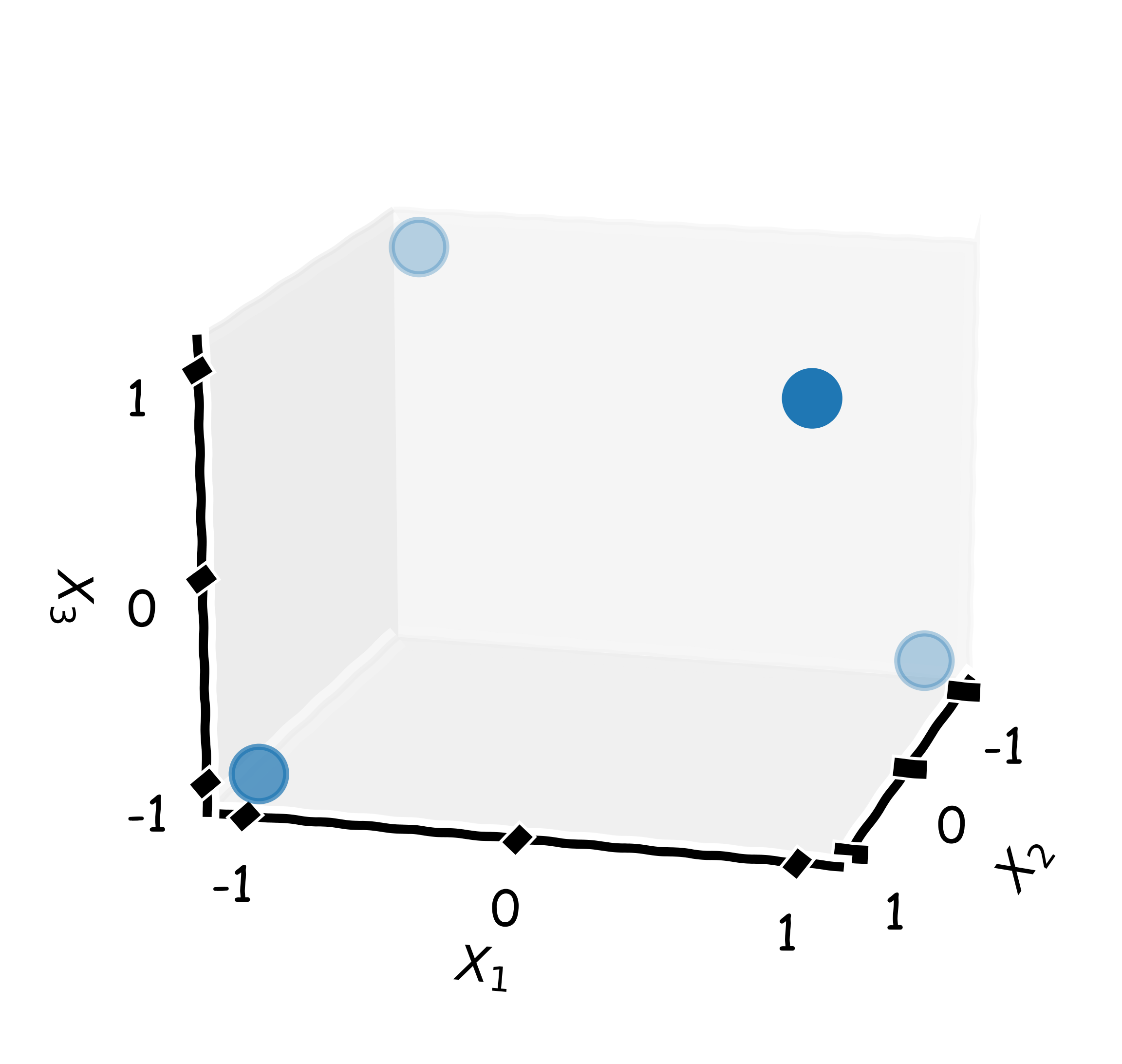
In fractional factorial designs (Fig. 1b), abbreviated as $2^{k-p}$, subsets of complete designs are used, in which some higher order interactions between variables are “aliased” with main effects or other higher order interactions. Aliasing is the phenomenon of lower and higher order effects becoming indistinguishable as they contain the same information, and the degree of aliasing is characterized by the resolution of a design (written in Roman numerals). The higher the resolution, the higher the order of interactions that can be estimated without aliasing them with lower order terms. To increase the resolution, more experiments need to be conducted, which enables determination of higher order effects acting on a system.
Aliasing and Resolution
To provide a better intuition for aliasing, a full factorial design for two variables $X_1$ and $X_2$ is depicted in the Tab. below.
| Experiment | $X_1$ | $X_2$ | $X_1 X_2 = X_3$ |
|---|---|---|---|
| 1 | $-1$ | $-1$ | $+1$ |
| 2 | $-1$ | $+1$ | $-1$ |
| 3 | $+1$ | $-1$ | $-1$ |
| 4 | $+1$ | $+1$ | $+1$ |
The last column covers the values for the interaction effect, which is obtained by multiplying $X_1$ with $X_2$. Suppose that a third variable $X_3$ should be added to the design; a full factorial design with three variables (and two levels) would contain eight experiments. Instead of adding four more experiments, it would be possible to use the configurations of the interaction term $X_1X_2$ for variable $x_3$. Therefore, $X_1X_2$ and $X_3$ would contain the same information, and it would be not possible to distinguish them (they are aliased). As a consequence, the interaction term would be omitted from the model. This is an example for a $2_{\text{III}}^{3-1}$ factorial design, i.e., three factors in one-half fraction with resolution III. If an interaction were negligible, this would be a reasonable design for a calibration model since four data points are available for four parameters (three factors and an intercept).
Alias Structure
The described concept can be extended to any set of variables {$X_1$, $…$, $X_k$}, whereas it is possible to specify the design resolution for a fixed number of variables to actively control the possible terms that can be included in the model. The collection of effects that are aliased with each other is called alias structure. For larger sets of variables, the alias structure becomes more complex but it should be tracked as it puts constraints on a linear model. Unintended aliasing should be avoided because it leads to wrong conclusions.
The alias structure is identified as follows. Let $\mathbb{I}$ be the identity vector (a vector with $+1$’s) with same dimension as any variable vector in the design. Properties of the orthogonal design matrix are ($\odot$ denotes the Hadamard, i.e., element-wise, product):
- Any column $\mathbf{x}_1$, $…$, $\mathbf{x}_k$ multiplied by itself results in the identity column $\mathbb{I}$, for instance, $\mathbf{x}_1 \odot \mathbf{x}_1 = \mathbf{x}_1^2 = \mathbb{I}$.
- Multiplying $\mathbb{I}$ with any column does not change the column, e.g., $\mathbf{x}_1 \odot \mathbb{I} = \mathbb{I} \odot \mathbf{x}_1 = \mathbf{x}_1$.
To obtain a fractional factorial design for $k$ factors, a full factorial design with $q$ factors is constructed, whereas $q < k$. The other $k-q$ factors are expressed as interaction effects of this base design, e.g., $X_4 = X_1X_2$, or $X_5 = X_1X_3$; those are the design generators, whereas $X_1X_2$, $X_1X_3$, and so on are referred to as “words”. Evidently, it is essential to choose a base design that is large enough to have sufficient interaction terms for the residual $k-q$ factors. Moreover, it holds that $\mathbb{I} = \mathbf{x}_1\odot \mathbf{x}_2 \odot \mathbf{x}_4$ and $\mathbb{I} = \mathbf{x}_1\odot \mathbf{x}_3\odot \mathbf{x}_5$, which is essentially the multiplication of the design generators with left-hand side of the equations; those are the so-called defining relations.
By multiplying these relations with any variable of interest, the aliases are obtained, e.g., $\mathbf{x}_1 \odot \mathbb{I} = \mathbf{x}_1 \odot \mathbf{x}_1\odot\mathbf{x}_2\odot\mathbf{x}_4 = \mathbf{x}_1^2\odot\mathbf{x}_2\odot\mathbf{x}_4 = \mathbf{x}_2\odot\mathbf{x}_4$. Hence, $X_1$ is aliased with $X_2X_4$, and it is impossible to differentiate between the main effect $X_1$ and the interaction $X_2X_4$. In general, the resolution of a two-level fractional factorial design is equal to the number of letters in the shortest word of the defining relations, and the highest possible resolution is found by using the interaction effects of the highest possible order as generators for additional variables.
-
D. Montogmery, Design and Analysis of Experiments, 8th Edition, Wiley. ↩