Blind Calibration

Introduction

Sensor networks have emerged as a technology that enables the monitoring and control of processes in manufacturing plants or smart cities. In the case of air quality monitoring in smart cities, for example, particularly polluted places could be identified in real-time and citizens protected from the effects of air pollution. Such networks consist of many distributed (gas, temperature, humidity, etc.) sensor nodes that collect data and transmit them to a central place where they can be processed.

These measurement systems, however, place new demands on calibration, e.g., in terms of scale and frequency. More precisely, these countless sensors are often of inferior quality and therefore need calibration more often. Manually calibrating each node or collecting all nodes and bringing them to a laboratory (for calibration) would be too tedious, if not impossible, and would also result in downtime and missing data. Still, calibrations are necessary because they make measurements comparable in space and time. If sensors drift, their measured values do not correspond to the truth. As a result, decisions based on such data will be unreasonable.

How to keep sensor networks calibrated has therefore been the subject of research, giving rise to so-called blind calibration algorithms (among other types of automated calibration techniques), which aim at improving the data quality of measurements of the sensors and delay (or even omit) expensive manual calibrations. Simply put, they use an initial calibration as a reference; the key idea is to exploit correlations between sensor signals, allowing to compute new calibration coefficients using techniques from linear algebra and mathematical optimization. This article explains the theory behind such algorithms and demonstrates their potential and limitations with a practical example.

Theoretical Background

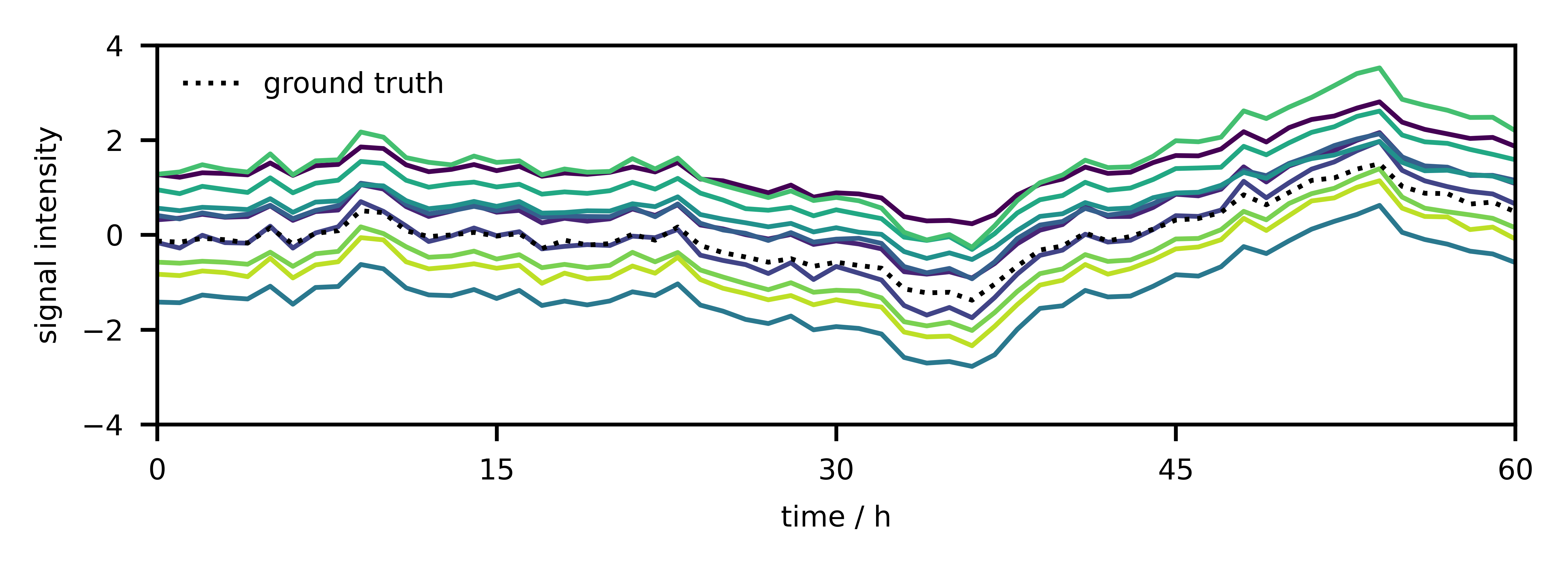
The starting point is a sensor network consisting of $n$ nodes, each sensing a certain process. At time $t$, the individual measurements are collected as in a vector $\mathbf{y} = [y_1, …, y_n]$. If the individual sensors “see the same thing”, their signals will be correlated to a large degree. Such correlation can happen if the phenomenon to be measured behaves similarly at different locations or all sensors are at the same location measuring the same or different processes that are coupled. As a consequence, the collection of measurements will lie in a subspace of dimensionality $r < n$. Although the sensors will be calibrated initially, gain $\alpha \in \mathbb{R}^n$ and offset $\beta \in \mathbb{R}^n$ drift (shown in Fig. 1) will make recalibration necessary (Eq. \ref{eq1}),

\begin{equation} x = \mathbf{Y}\alpha + \beta, \label{eq1} \end{equation}

with $\mathbf{Y}$ = diag($\mathbf{y}$).

If we learn the projection matrix $\mathbf{P}$ of dimensionality $n - r$ associated with the signal nullspace (i.e., the orthogonal complement to the signal subspace $\mathcal{S}$), we can try to estimate the correct gain and offset coefficients. The idea is that the true signals should remain in the signal subspace $\mathcal{S}$ at all times (Eq. \ref{eq2}),

\begin{equation} \mathbf{P}x = \mathbf{P}(\mathbf{Y}\alpha + \beta) = 0. \label{eq2} \end{equation}

The part of the drift in $\mathcal{S}$, however, cannot be recovered, so it must be assumed that the average signal has a zero mean. Note that too much noise destroys existing correlations. Another important prerequisite is that the basis is robust (the correlations have to persistent). This projection matrix $\mathbf{P}$ can easily be found by collecting measurements in an initial phase (in which the sensors have no drift at all) and by performing a principal component analysis.

Then, if we collect $k$ snapshots (Eq. \ref{eq3}),

\begin{equation} \mathbf{P}(\mathbf{Y}_i \alpha + \beta) = 0,\quad i = {1, …, k}, \label{eq3} \end{equation}

we can use them to compute the calibration factors (almost) blindly. The formula above holds for any $\mathbf{Y}$, in particular also for the average $\bar{\mathbf{Y}}$. From this observation, we can conclude that (Eq. \ref{eq4})

\begin{equation} \hat{\beta} = −\bar{\mathbf{Y}}\alpha. \label{eq4} \end{equation}

Inserting this expression for $\beta$, we obtain (Eq. \ref{eq5})

\begin{equation} \mathbf{P}(\mathbf{Y}_i−\bar{\mathbf{Y}})\alpha = 0,\quad i = {1, …, k}. \label{eq5} \end{equation}

The individual snapshots $\mathbf{P}(\mathbf{Y}_i−\bar{\mathbf{Y}})$ can be stacked in a matrix $\mathbf{C}$. Because the observations are noisy, we have to minimize a squared loss with respect to the gain vector $\alpha$ to obtain (Eq. \ref{eq6})

\begin{equation} \hat{\alpha} = \arg \min_{\alpha} \alpha^{T} \mathbf{C}^{T} \mathbf{C} \alpha \label{eq6} \end{equation}

with the constraint that $\alpha_1 = \alpha_{true}$, that is, we need to know at least one gain factor, but it does not matter which one. Alternatively, we could also fix any of the gains to $1$, and the other gains would be relative to this so-called global gain factor. Such a constraint can be interpreted physically to mean that all sensors are calibrated to the gain characteristics of the first sensor. The raison d’être for the constraint is that the solution will be $\hat{\alpha} = 0$ without it, which is not what we want.

One interesting question is how many snapshots to collect, i.e., what value to choose for $k$. For the gains, it holds that $k \geq \lceil \dfrac{n - 1}{n - r} \rceil$. Since the offsets are then computed from an average, more snapshots will generally lead to a more precise estimate.

Methods

Step 0: Get some data.

This example makes use of some chemical process data. One of the sensor readings is taken and replicated several times to simulate the sensor network. In addition, some noise is added, the signals are standardized. Finally, some drift is injected.

import pandas as pd
import numpy as np

# Load data.
data = pd.read_excel("Distillation Column Dataset.xlsx", index_col=0)
data.index = pd.to_timedelta(data.index, unit="seconds")
data = data.rolling(window="600 s").mean()

# Create replicate sensor data (to have correlations).
n_sensors = 10
S = np.repeat(np.expand_dims(data.Sensor1.values, 
                             axis=0), 
              repeats=n_sensors, axis=0).T
S += np.random.normal(0.0, 0.002, S.shape)  # add some noise

# Standardize data.
scaler = StandardScaler()
X = scaler.fit_transform(S)

# Let sensor data drift.
_, n = X.shape
slope = np.random.normal(1, 0.2, size=(n))
intercept = np.random.normal(0, 1.0, size=(1, n))
X_drift = np.add(np.multiply(X, slope), intercept)

Step 1: Finding the subspaces.

The subspaces are found by principal component analysis. Because the signals replicates, it suffices to set $r = 1$. In the general case, however, this needs to be determined experimentally.

from sklearn.preprocessing import StandardScaler
from sklearn.decomposition import PCA

_, n = X.shape  # get shape of sensor data set
pca = PCA(n_components=n, random_state=0)
T = 300  # duration of initial calibration
pca.fit(X[:T, :])  # fit pca on calibrated sensor data

r = 1  # pick dimensionality of r
P = pca.components_[r:, :]  # extract projection matrix

Step 2: Taking snapshots.

In a next step, $k = 10$ snapshots are taken.

T_s = 301  # when to start taking snapshots
k = 10  # number of snapshots
Y = X_drift[(T_s):(T_s+k), :]
Y_bar = np.mean(Y, axis=0)  # compute average snapshot

# Construct data set.
C = np.zeros((k*(n-r),n))
for i in range(k):
    C[i*(n-r):(i+1)*(n-r),:] = (P @ (np.diag(Y[i,:]) - np.diag(Y_bar)))

Step 3: Calibrating the gains.

To calibrate the gains, the constrained optimization problem is solved.

from scipy.optimize import minimize, NonlinearConstraint

# Define some variables.
n_variables = n
n_constraints = 1

# Define objective function.
def objective(a):
    return (a.T @ C.T) @ (C @ a)

# Define constraints.
def system(a):
    return a[0] - 1/gain[0]  # we need to know at least one gain
nonlinear_constraint = NonlinearConstraint(system, 
                                           np.zeros((n_constraints)), 
                                           np.zeros((n_constraints)))

# Define starting point of optimization.
a0 = np.ones((n_variables))

# Run optimization.
res = minimize(objective, a0, method="trust-constr",
               constraints=[nonlinear_constraint],
               options={"verbose": 1, "maxiter": 50000},
               tol=1e-20)
gains = res.x

Step 4: Calibrating the offsets.

Having obtained the gains, the offsets can be computed.

# Get offsets.
offsets = np.zeros((n))
for i in range(n):
    offsets[i] = - gains[i] * Y_bar[i]

Results

Fig. 2 illustrates the original signals and the ones after blind calibration. It becomes clear that the drift could be almost completely eliminated. In addition, the correct signal was restored because the individual signals overlapped with the dashed line.

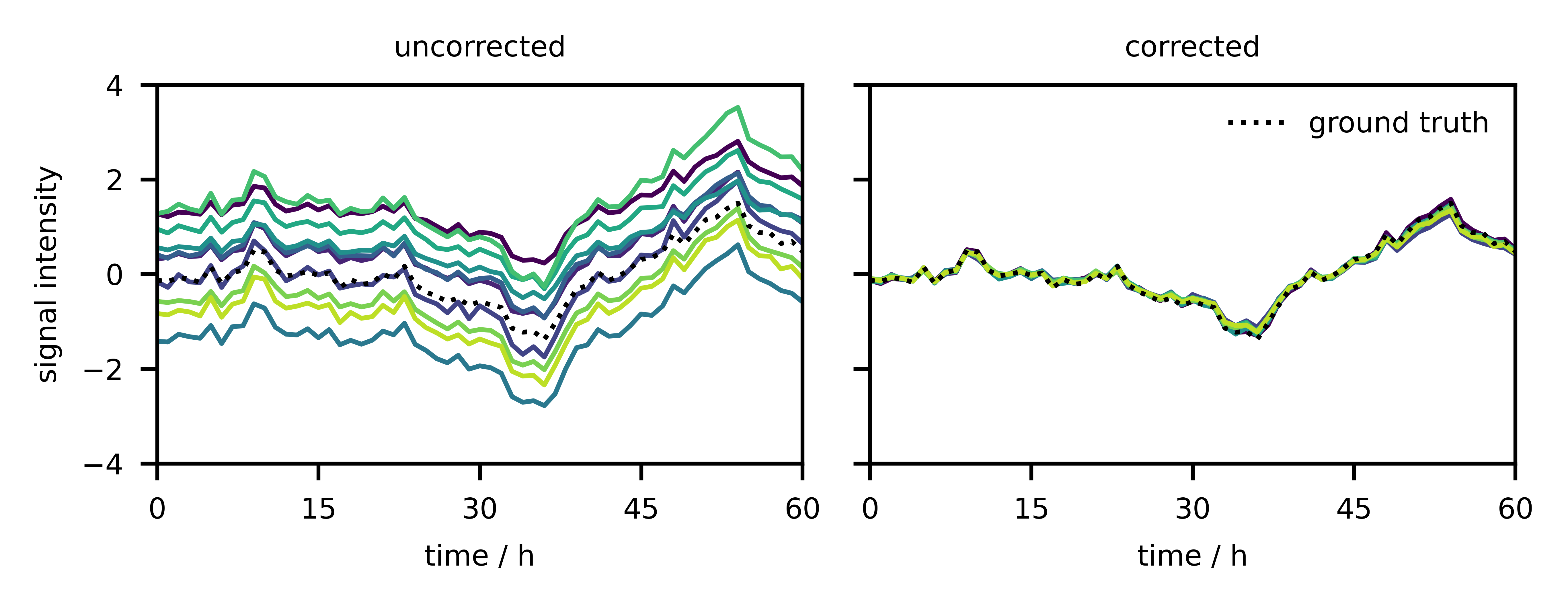
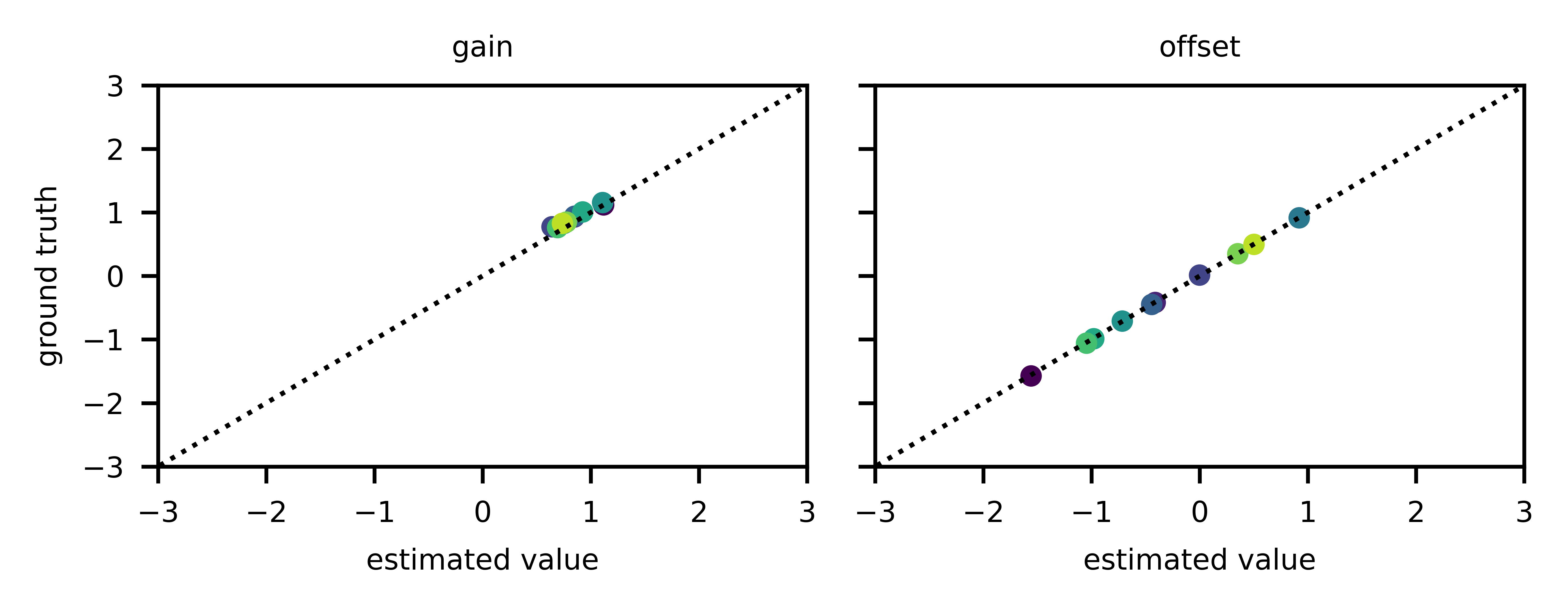
Fig. 3 relates the estimated gains and offsets to the correct ones. By and large, the parameters match, although a slight mismatch can be observed in the gain.

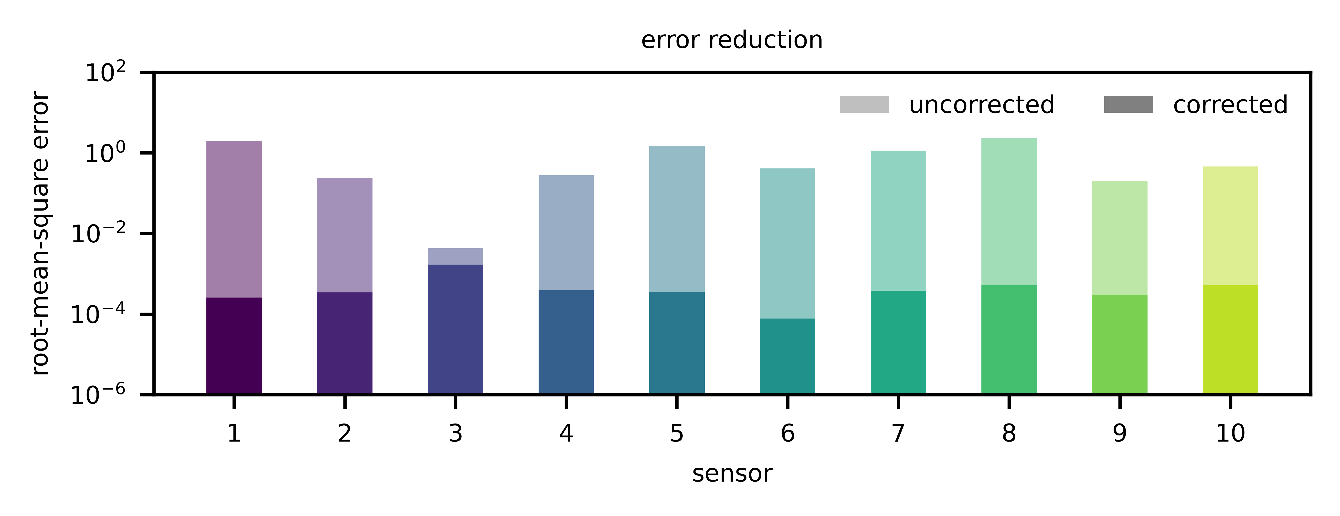
Finally, Fig. 4 compares the improvement of the measurement with respect to the root-mean-square error. Here we can clearly see that the improvement is not negligible.

Conclusion

This article has shown the benefit of blind calibration. This idea has evolved over time and lead to a class of algorithms that can also be used to estimate drift and subtract it from the signal. Nevertheless, the approach is not suitable for all sensor networks. First and foremost, the correlation assumption must be given. For this reason, the data quality must be sufficient, otherwise the correlations will break apart. In addition, the projection matrices must remain stable over time, which is not always the case. Finally, the signal must average out over time, i.e., its mean must be zero. For all other cases, alternatives have been developed, for example calibration by means of mobile references, but this requires that high quality references can be produced inexpensively, for example using automated laboratory calibrations.